Microstructure Lectures

Table of Contents:

1. Introduction
2. Cracks: Atomistic - at Interfaces - in a Continuum
3. Cracks Near Interfaces Between Dissimilar Isotropic Materials
4. Introduction to Mechanical Behavior of Anisotropic Laminates
   • 4.1 Introduction to Mechanical Behavior of Anisotropic Materials
   • 4.2 Introduction to Mechanical Behavior of Laminates
5. Laminate Singularities Caused by Anisotropy: "Free-Edge Problem"
6. Laminate Singularities Caused by Ply Cracks
7. Cracks Near Interfaces Between Dissimilar Anisotropic Materials
   ------ Extension to a Homogeneous Continuum ------

8. Cracks in Homogeneous Isotropic Materials
9. Cracks in Homogeneous Anisotropic Materials
10. Wave Propagation in Homogeneous Isotropic/Anisotropic Materials
11. References

---

7.0 Cracks Near Interfaces Between Dissimilar Anisotropic Materials

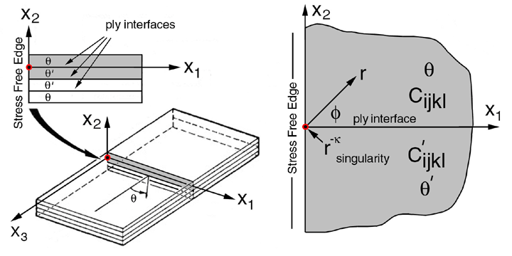
In previous sections we studied stresses near laminate stress free edges and ply cracks that exist at an interface between two dissimilar anisotropic materials. These results were predicted by a Finite Element Model (FEM) that did not include singularities. Instead stresses gradients near the free edge and ply crack tips were approximated with a high density FEM mesh near the singurality. In this section we introduce an analytic model that predicts these singularites: 7.1) at a bimaterial interface intersecting a stress free edge, see Figure 30, and, 7.2) at a ply crack tip intersecting an interface seperating two dissimilar anisotropic media, see Figure 31. Both models are solved using Stroh's method, Ref.[24]. These singularites can be introduced into enriched FEMs that included a variety of different boundary conditions (BCs) without using high density FEM meshes. With these enriched FEMs, stress intensity factors can be solved for as unknowns along with the nodal displacements for each unique geometry and BCs. Section 8 will outline how to create a finite element model with elements "enriched" with these singularities.

For both models, shown in Figs. 30 and 31, it is important to note that the singularity coincides with the origin of the coordinates. Hence each model has a unique coordinate system. Since the objective here is to reproduce published results of these two models the same coordinate system established by Ting et al. will be used. This choice will require rederivation of an arbitray rotation in the 1-2 plane for orthorhombic symmetry outlined in section 4.1. The derivations below will follow the notation and procedures outlined by Ting et al, Refs. [25] and [26]. The notes below will expand on the solution introduced by Ting et al. by developing the numerical approach to solve for these singularities.

7.1 Stress free edge singularities:

Figure 30. Coordinates defined for stress free edge singularity Ref.[25].

T.C.T. Ting and S.C. Chou, Ref.[25], used Stroh's method to solve for the singularity where the interface seperates two dissimilar anisotropic regions and terminates at a stress free edge, see Figure 30. Here we only expand on the development of the numerical solution and use the same notation in Ref.[25] except the exponent on the radius, r, is changed from, d, to -k similar to the exponent in Ref.[26].

The solution is organized into three parts: 1) transformation of the fourth order stiffness tensor, C_ijkl, for arbitrary rotation in the 1-3 plane, see eqn 35 Ref.[25], 2) calcuate eigenvalues, p_k, and eigen vectors, n_i and t _ij, from equations (9) and (10) Ref.[25], and 3) calcuate exponent (singularity) on radius, r, from the determinate of equations that are created when equations (30) and (31) of Ref.[25] are combined with appropriate boundary conditions.

7.1.1 Tensor Transformation C_ijkl in 1-3 plane:

Hand-written notes are provided for the transformation of the fourth order stiffness tensor for arbitray rotations in the 1-3 plane.

7.1.2 Calculate Eigenvalue/Eigenvectors, p_k / n_i and t_ij:

We start with equations (9) and (10) in Ref.[25].

(9) Ting

(10) Ting

where

(11) Ting

(12) Ting

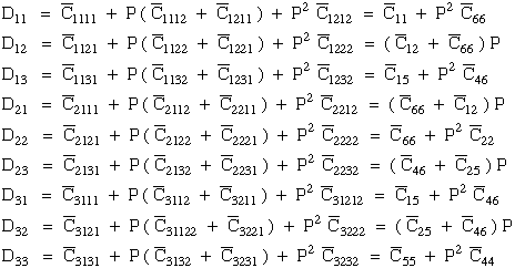
Below we expanded and simplify eqn. (10) into an eigenvalue problem that we can solve by using IMSL scientific subroutines. Combining equations (11) and (12) from Ref.[25] along with the rotated transformed stiffnesses, yields

(67)

where

(68)

Substituting eqn (68) into eqn (10) of Ref.[25] yields

(69)

Note that P_L exists in every term of the coefficient matrix in eqn. (69) who's determinate yields a cubic characteristic equation in P_L². Although it is possible solve for the roots of this characteristic equation, numerical solutions to this type of problem yield more accurate eigenvalues. Hence eqn.(69) is further developed into an eigenvalue problem where P_L are complex eigenvalues and their corresponding complex eigenvectors, n _i,L, where the ,L subscript associates the eigenvector with the appropriate eigenvalue (L=1,2,3). The L is not a free indice and the comma does not imply differentiation

The eigenvalue format is

(70)

It is possible to expand equation (69) into the form of equation (70). First we rewrite equation (69).

(71)

where we can write equation (71) in abbreviated notation.

(72)

Multiply equation (72) by the inverse of the coefficient matrix, [A'], yeilds.

(73)

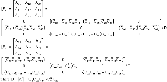
where [A']^-1[A'] becomes the indentity matrix [I], and matrices [B'] and [C'] are premultiplied by [A']^-1 and become [B] and [C] respectively.

(74)

The array [A] in eqn.(70) can be constructed such that

(75)

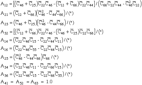
where the nonzero components in array [A] of eqn.(70) are summarized below.

(76)

To show eqn.(70) and eqn.(73) are equivalent requires the following expansion. First substitute eqn.(75) into eqn.(70) where the {Z} eigenvectors are partioned into X_i and Y_i components.

(77)

where

(78)

Equation (77) can be rewritten interms of X_i and Y_i components.

(79)

Expanding eqn.(79) yields two equations

(80)

These two equations can be combined into one equation by substituting for X_i, hence eliminating X_i, and rearranging terms.

(81)

where comparing equations (81) and (73) yield the necessary eigenvalues and eigenvectors

(82)

Comparing equations (81) and (73) verifies that equation (70) can be used to solve for P_L as eigenvalues instead of roots to the characteristic equation derived from the determinate of the coefficient matrix in equation (69). Both eigenvalues, P_L, and eigenvectors from equation (81) will be used in the next section to calculate the singular exponent. IMSL routines EVCRG are used to solve equation (70) and EPIRG is used to obtain a performance index for the solutions.

7.1.3 Calculate Singular Exponent, -k:

Using Stroh's method Ting et al., Ref.[25], obtained the functional form for displacements and stresses.

(30) Ting

(31) Ting

where again we note that ,L does not imply differentiation and L is not a free indice but is used as a subscript to identify eigenvectors associated with the L-th eigenvalue. Here L is assigned 1,2,3 corresponding to the three eigenvalues of eqn.(69).

(26) Ting

The equations above have been slightly modified. The exponent has been changed from d to -k and the coefficients, M_L and N_L have been renamed a_L and a'_L.

To solve for the exponent singularity, k, we create a systems of 12 linear equations from Ting's equations (30) and (31) and the boundary conditions listed below. Coefficients of these equations are written in terms of k and solved for k as a root to the determinate of the coefficient matrix of these equations. Since the solution is to find only one of the roots between 0.0 and 1.0, this root is first approximated by calculating the determinate as a function ("function-subroutine") of k where a value for k is incremented from 0.0 to 1.0 until the determinate changes sign (+/-). Within this interval a root exists. With an approximation for the root interval other IMSL routines can be used to obtain a more accurate solution for k. Next we construct the twelve equations for the boundary conditions defined in Fig. 30.

The boundary conditions are:

(83)

From these boundary conditions 12 equations are generated whose coefficients are functions of elastic properties and the exponent on the radius vector whose origin is located at the crack tip where the singularity exists. Below we generate this coefficient matrix.

Boundary condition 1:   

(84)

Boundary condition 2:   

(85)

Boundary condition 3:   

(86)

Boundary condition 4:   

(87)

The blocks defined above are substituted into the schematic shown below.

Figure 30. Block schematic of system of equations for determining singularity
where bimaterial interface terminates at a stress free laminate edge.

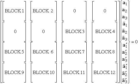
IMSL routine ZBREN is used to find a solution (root) to the determinate of the coefficient matrix shown in Fig. 30. The ZBREN requires an initial guess where the determinate changes sign in the interval from 0 to 1.0. Hence a function subroutine, F, is setup which calculates the determinate using IMSL routines LFTRG and LFDRG.

• Interactive Computer Program: Experiment with Singularities at Interfaces Between Dissimilar Anisotropic Materials at a Stress Free Laminate Edge: Analytic Model (Stroh's Method)

With the interactive computer program provided above the student can reproduce the singularities tabulated below. In particular the default values set in the NPIB form of the computer program is configured to calculate the singularity of 2.9388 x 10^-2 for q'=0 and q'=75 with the Pipes-Pagano approximation for elastic properties:

E₁=E₂=+2.100E+06,    E₁=+2.000E+07
G₁₂=G₁₃=G₂₃=+0.850E+06
n₂₁= n₃₁= n₃₂=+0.210E+00

7.2 Ply Crack singularities:

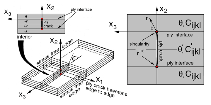
T.C.T. Ting and Hoang, Ref.[26], used Stroh's method to solve for the singularity at a ply crack tip acting normal to an interface seperating two dissimilar anisotropic regions, see Figure 31.

It is important to note that singularities coincide with the coordinate system origin. Hence each interface singularity has a unique coordinate system. Since the objective here is to reproduce published results the same coordinate system established by Ting et al. will be used. This choice will require rederivation of an arbitray rotation in the 1-2 plane for orthorhombic symmetry outlined in section 4.1. The derivations below will follow the notation and procedures outlined by Ting et al, Refs. [26]. For this module we have expanded on the solution introduced by Ting et al. and developed the numerical approach to solve for these singularities.

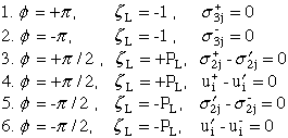
The solution is organized into three parts: 1) transformation of fourth order stiffness tensor, C_ijkl, for arbitrary rotation in the 1-3 plane, see eqn 35 Ref.[25], 2) calcuate eigenvalues, p_k, and eigen vectors, n_i and t_ij, from equations (9) and (10) Ref.[25], and 3) calcuate exponent, k (singularity) on radius, r, from determinate of equations that are created when equations (21) and (22) of Ref.[26] are combined with the appropriate boundary conditions equation (36) of Ref.[26]. NOTE: The geometry shown in Fig.31 results in a set of boundary conditions different then those used in the previous section 7.1.

(88)

From these boundary conditions 18 equations are generated. Coefficients are functions of elastic properties and the exponent on the radius vector whose origin is located at the crack tip where the singularity exists. Unlike boundary conditions for the free edge problem of section 7.1, there is an additional notation where + or - appear as superscripts on variables that indicates these variables exist in regions x₃ > 0 and x₃ < 0 respectively.

Partial results from Ting et al. Ref.[26] are listed below in Table 1 with the Pipes-Pagano approximation for elastic properties:

E₁=E₂=+2.100E+06,    E₁=+2.000E+07
G₁₂=G₁₃=G₂₃=+0.850E+06
n₂₁= n₃₁= n₃₂=+0.210E+00

We provide an interactive computer program module below where you can reproduce these results. The default values in the NPIB form will generate results highlighted in red in the Table above for q'=30 and q'=60 which uses the Pipes-Pagano approximation for elastic properties.

• Interactive Computer Program: Experiment with Singularities at Ply Cracks that Terminate Normal to Interfaces Between Dissimilar Anisotropic Materials: Analytic Model (Stroh's Method)